
Asynchronous & Mixed-Shutter Cameras
Unsynchronized multi-camera VIO — epoch-anchored cloning, the ACI² preintegration bridge, and rolling-shutter support.
Classical multi-camera VIO assumes hardware-synchronized cameras: every camera exposes at the same instant, so one filter clone serves all of them. voxl-open-vins-server removes that requirement. Cameras may free-run at different rates with arbitrary phase, and each camera may be global- or rolling-shutter — including rigs that mix a rolling-shutter hires sensor with a global-shutter tracking camera. Synchronized rigs run the identical code path, unchanged.
This page explains the three mechanisms that make it work: the lock-free ingest, epoch-anchored cloning with the ACI² preintegration bridge, and the per-row rolling-shutter measurement model.
Table of contents
- Why unsynchronized cameras are hard
- Lock-free asynchronous ingest
- Epoch-anchored cloning and the ACI² bridge
- Rolling-shutter support
- Mixed-shutter rigs and the
fpvhiresconfiguration - Estimation quality on asynchronous rigs
- Configuration reference
- Further reading
- Appendix — mathematical reference
Why unsynchronized cameras are hard
Feeding unsynchronized cameras to a stock MSCKF filter fails in one of two ways:
Snapping timestamps (pretending frames are synchronized) injects a systematic timing error of up to half a frame period. At a focal length of 450 px and a rotation rate of 1 rad/s, a 7 ms phase error is a ~3 px systematic reprojection bias against a ~1 px noise model. The filter cannot tell timing error from calibration error, so it slowly corrupts its own calibration and bias estimates until it diverges.
Cloning at every camera’s frame time fragments the filter’s sliding window. With N cameras, each camera’s feature tracks only span 1/N of the window, so tracks hit the marginalization horizon early, never reach the length that promotes them to SLAM landmarks, and triangulation loses its baseline. The estimator starves.
The resolution is to keep one clone timeline — anchored to a single reference camera — and to attach every other camera’s measurements to that timeline exactly, using the IMU itself.
Lock-free asynchronous ingest
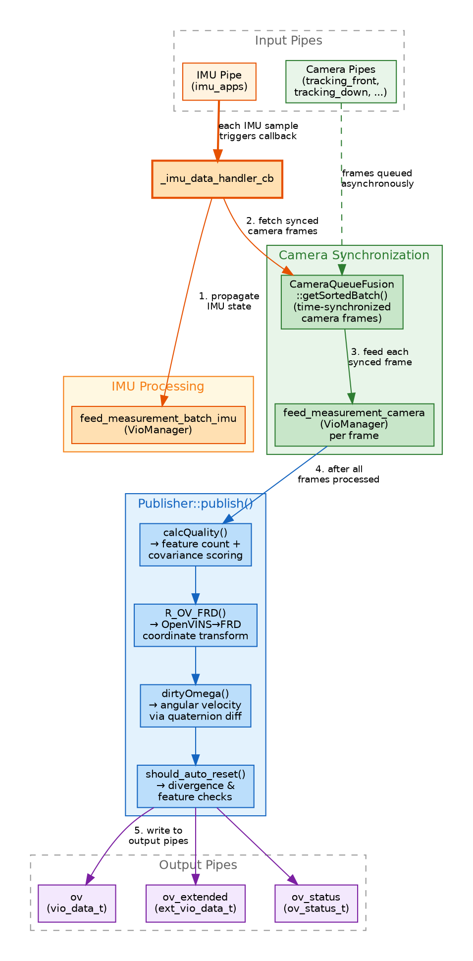
Every camera owns a lock-free single-producer/single-consumer ring inside the estimator. Camera pipe callbacks push frames and return immediately — no locks, no fusion thread, no pairing logic. The IMU callback (the single VIO thread) releases frames when three conditions hold:
- IMU coverage — inertial data spans past the frame time (plus a small guard), so propagation never extrapolates;
- global order — every other live camera has either delivered a frame at or beyond this time, or has been silent long enough (relative to its own measured frame period) that it cannot block;
- per-stream order — frames that arrive out of order or too late are dropped, and every dropped frame is released back to its owner exactly once.
A dead or throttled camera therefore adds bounded latency instead of stalling VIO, and a healthy rig holds all drop counters at zero.
The staleness gate is self-tuning: each stream maintains an exponentially-weighted moving average of its own frame period, updated on every arrival (90/10 blend — see Appendix A.4). The declared per-camera frame rate (camN_fps, below) seeds this EMA, so the ordering gates run at design width from the very first frame after boot and after every reset instead of converging over a warm-up window.
Epoch-anchored cloning and the ACI² bridge
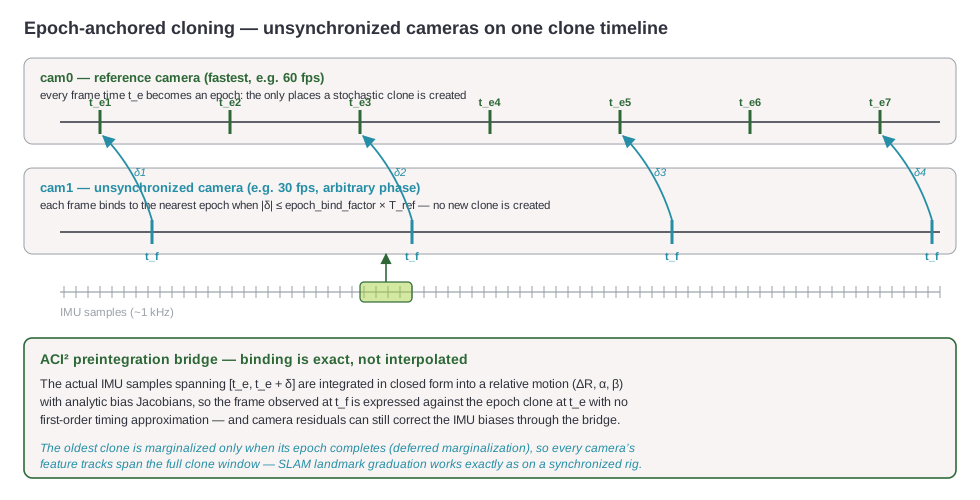
With epoch_mode enabled, stochastic clones are created only at the reference camera’s frame times — the epochs. When another camera’s frame arrives at time t_f, its known offset from the preceding epoch, δ = t_f − t_e (non-negative, since frames are released in global time order), is bridged with an ACI²-style closed-form preintegration of the actual IMU samples spanning [t_e, t_f]: a relative rotation ΔR and position/velocity preintegrals α, β that express the camera pose at t_f exactly in terms of the epoch clone at t_e.
Two properties make this a first-class filter update rather than an approximation:
- Exactness — the bridge integrates real IMU data in closed form; there is no first-order “pose interpolation” error, no matter where in the frame interval the measurement falls.
- Analytic bias Jacobians — the bridge carries
∂(ΔR, α, β)/∂(b_g, b_a), so camera residuals on bridged frames still correct the IMU biases through the bridge, preserving the estimator’s observability structure and consistency (first-estimate Jacobians throughout).
The reference camera must be the fastest camera. A slower reference forces the faster camera to deliver more than one frame per epoch; the extras fall back to private clones and the window fragments — exactly the failure epoch mode exists to prevent. The server warns at boot if the declared rates violate this.
Deferred marginalization. An epoch’s measurements arrive in installments — the reference frame first, bound frames up to one binding horizon later. The oldest clone is marginalized only when its epoch completes, so every camera’s tracks span the full clone window and SLAM landmark promotion behaves exactly as on a synchronized rig.
Rolling-shutter support
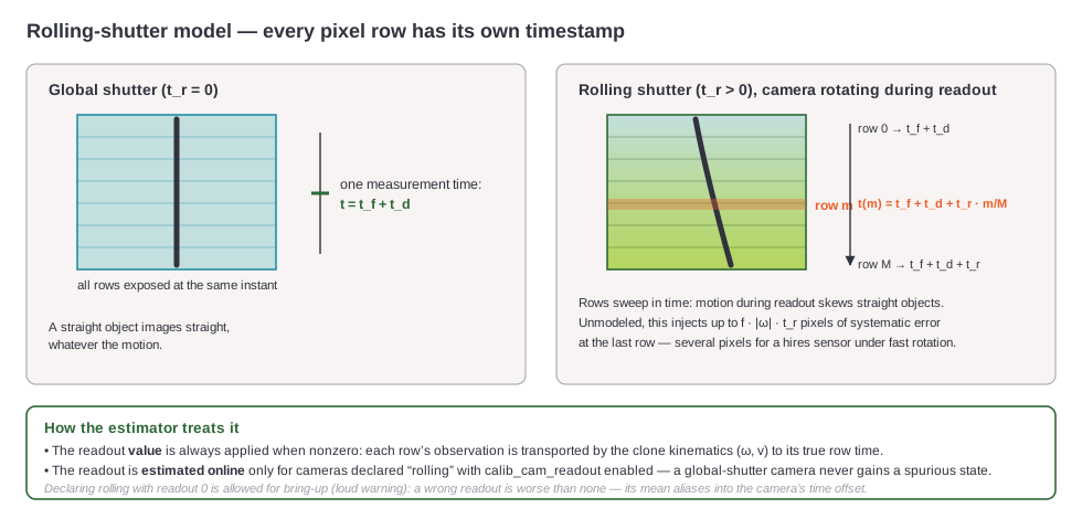
A rolling-shutter sensor exposes row by row. Since SDK 1.8.0 (server 0.7.8) every frame stamp is the center row at mid-exposure, applied once at ingest (t_frame = HAL3 start-of-frame + (t_readout + exposure)/2), and a pixel on row m of M was imaged at
t(m) = t_frame + t_offset + t_readout · (m/M - 0.5)
The row anchor is the estimator key rs_convention, which drives both the stamp anchoring and the filter’s row model so the two cannot disagree:
rs_convention | Frame stamp | Row time |
|---|---|---|
center (shipped profiles) | SOF + (readout + exposure)/2 | stamp + (m/M - 0.5) · readout |
top | raw HAL3 start-of-frame | stamp + (m/M) · readout |
bottom | SOF + readout + exposure/2 | stamp + (m/M - 1.0) · readout |
Server builds before 0.7.2 stamped frames at the raw start-of-frame and used the top-anchored model (t_readout · m/M). A camera chain calibrated under that convention carries the anchor difference inside its timeshift_cam_imu until it is recalibrated.
The estimator applies this per measurement row: each observation is transported to its true row time using the clone’s angular and linear velocity. Two rules keep this safe:
- Value vs. estimation. The readout value is always applied when nonzero. It is the HAL3 hardware readout of the streamed sensor mode and is not calibrated: every shipped rolling-shutter profile sets
calib_cam_readout: false. Online readout estimation is only possible for cameras explicitly declared"rolling"; a global-shutter camera’s readout stays pinned at zero and never becomes an estimated state. - Degenerate-motion gating. Temporal parameters (time offsets, readout) are only observable when the motion varies. Under hover or constant-velocity cruise the estimator freezes their estimation (values remain applied) rather than letting them drift on noise.
A wrong readout value is worse than none. The row-averaged part of a readout error is indistinguishable from a camera time offset and will silently bias it, while the row-dependent part corrupts calibration. Measure the readout of the streamed sensor mode (rows × line time) rather than guessing from a datasheet; if you cannot measure it yet, declaring the camera
rollingwith readout0runs the sensor deliberately unmodeled with a loud boot warning — a legitimate bring-up state.
Mixed-shutter rigs and the fpvhires configuration
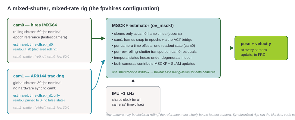
The mechanisms above compose: a rolling-shutter hires camera and a global-shutter tracking camera, at different rates, with no sync line, share one clone window and both contribute MSCKF and SLAM updates. That is the fpvhires configuration:
voxl-configure-open-vins fpvhires
which points the server at the /usr/share/modalai/voxl-open-vins/VoxlConfig/fpvhires estimator configuration — IMX664 hires (rolling shutter, 60 fps, epoch reference) plus AR0144 tracking (global shutter, 30 fps) with epoch_mode enabled — and sets sync_config: true, so the OpenVINS calibration YAMLs are regenerated from your system calibration at every startup. (sync_config only controls this calibration synchronization; frame ingest is always the lock-free asynchronous path, and whether frames share timestamps is a property of the rig, not a configuration switch.)
Because
fpvhiressynchronizes calibration from the system at startup, your system calibration must be complete and correct before enabling it:
- Intrinsics — both cameras calibrated, with their calibration files present in
/data/modalai/(see Camera Calibration).- Extrinsics —
/etc/modalai/extrinsics.confmust contain thebody → imuand camera relationships for both the hires and the tracking camera (see Configure Extrinsics)./etc/modalai/vio_cams.conf— edit it so exactly these two cameras are enabled: the hires camera’spipe_for_tracking(e.g. the hires grey/misp stream) and the tracking camera’s pipe, each with the correctcal_file, and both referencing the sameimu.With any of these missing or stale, the regenerated calibration will be wrong and the estimator will misbehave in ways that look like tracking problems.
The classic synchronized configurations (fpv, starling2_2cam, …) are untouched and keep running the synchronized path.
Hardware-synced AR0144 tracking cameras
Since SDK 1.8.0 the released package handles hardware-synced AR0144 pairs through the estimator key force_camera_sync. It groups the dual-mono frames on their hardware exposure-start stamp and gives both views the center timestamp of the cam_imu_dt_ref_camid camera. The shipped fpv, fpvM and starling2 profiles set force_camera_sync: true. It does not enable hardware sync in voxl-camera-server; the cameras must already share a trigger.
SDK 1.6 and older: synced-timestamp AR0144 support is not in the released package. For those SDKs, build the server from source on the target from the
masterbranch of the voxl-open-vins-server repository or, for epoch-synced AR0144 tracking cameras, thesynced-timestampbranch.
Estimation quality on asynchronous rigs
The published quality score (see the Pipe Interface page) needs special care on asynchronous rigs. Updates arrive per camera — the reference camera opens an update, the other camera’s features join up to a binding horizon later — and MSCKF features only surface in an update when their tracks end. Scoring any single update therefore sees a sparse, noisy sample of tracking health: half the rig on reference ticks, nothing at all on zero-velocity ticks. (A synchronized rig never noticed, because every update carried both cameras at once.)
The server solves this with a windowed union + EMA design:
- Pool every update’s used-feature list from the last 120 ms and de-duplicate by feature id — this reconstructs the full per-camera track set that a synchronized batch would have carried (and it is the horizon over which a dead camera’s evidence naturally ages out);
- Score each camera over the pooled set with the standard scorer — a 5×5 image-coverage grid combined with per-feature weights (SLAM landmarks by covariance and track quality, MSCKF tracks by quality and track length);
- Sum across cameras and clamp to 100 — identical fusion to the synchronized path;
- Smooth the published value with a 250 ms time-constant EMA: a single weak update moves the score by a couple of points, while a real tracking collapse still reaches the reset thresholds in about half a second.
The quality state is invalidated on every reset (sensor time is continuous across resets, so smoothed values from the previous estimation episode can never pre-charge the new one), and the score is capped low during initialization so a freshly built covariance cannot report false confidence. Exact formulas in Appendix A.5.
Configuration reference
All keys live in the selected estimator_config.yaml. Per-camera declarations tell the estimator what each physical camera is; they are validated at boot and the server fails fast on contradictions.
Per-camera declarations
| Key | Example | Meaning |
|---|---|---|
camN_shutter | "rolling" / "global" | Authoritative shutter type. global: readout forced to 0, never estimated. rolling: rolling-shutter model active whenever the readout value is nonzero |
camN_readout_time_s | 0.0058 | Sensor readout time (first→last row, seconds) of the streamed mode. Overrides any t_readout in the kalibr chain. Must satisfy t_readout ≤ 1/fps |
camN_fps | 60.0 | Nominal rate of the streamed mode; 0 or absent means undeclared (no gate seeding, no readout bound). When positive: seeds the ingest ordering gates and the epoch binding horizon from the first frame; used to sanity-check the readout and the reference-camera choice |
Asynchronous multi-camera keys
| Key | Default | Meaning |
|---|---|---|
epoch_mode | false | Enable epoch-anchored cloning. false preserves the classic synchronized behavior exactly |
cam_imu_dt_ref_camid | 0 | The reference (clock/epoch) camera — must be the fastest |
epoch_bind_factor | 1.2 | Binding horizon in reference frame periods: a frame binds to the preceding epoch when 0 ≤ t_f − t_e ≤ this many reference periods |
epoch_bridge_bias_cols | true | Analytic IMU-bias Jacobian columns on bridged measurements |
async_ring_size | 16 | Per-camera ingest ring capacity (frames) |
async_guard | 0.002 | IMU coverage guard (seconds) before a frame is released |
async_stale_factor | 1.5 | A camera silent longer than this multiple of its own frame period cannot block release ordering |
force_camera_sync | false | SDK 1.8.0+. Group hardware-synced frames on the exposure-start stamp and give every view the reference camera’s center timestamp. true in the shipped fpv, fpvM and starling2 profiles |
async_frame_clones | false | SDK 1.8.0+, opt-in. false in every shipped profile |
physical_camera_clones | false | SDK 1.8.0+, opt-in physical warm start. Global-shutter cameras with fixed calibration only; a rolling-shutter camera is rejected at startup. false in every shipped profile |
Rolling-shutter / temporal calibration keys
| Key | Default | Meaning |
|---|---|---|
calib_cam_timeoffset | — | Estimate per-camera time offsets online (offsets are read per camera from the kalibr chain’s timeshift_cam_imu) |
rs_convention | center | SDK 1.8.0+. Rolling-shutter row anchor and frame-stamp anchor: top, center or bottom (see Rolling-shutter support). Every shipped profile sets it explicitly |
calib_cam_readout | false | Refine the readout online (declared-rolling cameras only). false in every shipped rolling-shutter profile: the readout is the HAL3 hardware value |
calib_cam_readout_init_sigma | 0.001 | Initial 1-σ prior on an estimated readout (s). Use ~0.005 when starting from a datasheet-grade guess |
dt_calib_gate | false | Opt-in freeze of time-offset/readout estimation under degenerate motion (values remain applied) |
dt_calib_gate_min_omega | 0.10 | Gate threshold: window peak angular rate (rad/s) |
dt_calib_gate_min_vel_spread | 0.10 | Gate threshold: window velocity spread (m/s) |
Runtime telemetry: with debug verbosity the estimator prints a per-update
[EPOCH]line — epochs snapped vs. fallbacks, plus ingest drop counters (late / ring-full / bogus). On a well-configured rig fallbacks and all drop counters stay at zero; a climbing fallback count almost always means the reference camera is not the fastest declared camera.
Further reading
The full mathematical specification — the bridge closed forms and bias Jacobian recursions, the rolling-shutter Jacobians, the measurement-noise analysis, and the consistency validation — lives with the source in ov_msckf/README_ASYNC.md in the ModalAI OpenVINS fork. Server-side integration is in the voxl-open-vins-server repository.
Appendix — mathematical reference
Notation follows OpenVINS: JPL quaternions, with \({}^{I}_{G}R\) the rotation taking a vector from the global frame into the IMU frame, \({}^{G}p_I, {}^{G}v_I\) position and velocity, \(b_g, b_a\) the gyro/accel biases, and \(\lfloor\cdot\rfloor\) the skew operator.
A.1 Time model and epoch binding
A pixel on row \(m\) of \(M\), in a frame stamped \(t_{f,i}\) by camera \(i\) with time offset \(t_{d,i}\) and readout \(t_{r,i}\), was imaged at
\[t(m) \;=\; t_{f,i} + t_{d,i} + t_{r,i}\,\big(\tfrac{m}{M} - a\big) ,\]with row anchor \(a\) = 0.5 for rs_convention: center (the shipped profiles), 0 for top and 1 for bottom.
With epochs at the reference camera’s frame times \(t_e\), a frame’s epoch residual and the binding rule are
\[\delta_i \;=\; \underbrace{\big(t_{f,i} - t_e\big)}_{\text{raw, stored}} \;+\; \Delta t_{d,i} , \qquad\text{bind} \iff 0 \le t_{f,i} - t_e \le \beta\, T_{\mathrm{ref}} ,\]with \(\beta\) = epoch_bind_factor and \(T_{\mathrm{ref}}\) the reference frame period. The ordered ingest release makes the raw residual non-negative, so binding is one-sided (a frame binds to the epoch that precedes it). The raw part is stored per (clone, camera); the calibration part \(\Delta t_{d,i} = t_{d,i} - t_{d,r}\) is applied at update time, so the transport stays differentiable in the estimated time-offset states. One frame per (camera, epoch); a frame outside the horizon falls back to its own clone.
A.2 ACI² preintegration bridge
The bridge relates the IMU pose at the true imaging time \(t_f = t_e + \delta\) to the epoch clone by integrating the actual IMU samples over \([t_e, t_f]\) into relative terms \(\Delta R, \alpha, \beta\) (all expressed in the epoch frame):
\[{}^{I_f}_{G}R = \Delta R\; {}^{I_e}_{G}R, \qquad {}^{G}p_{I_f} = {}^{G}p_{I_e} + {}^{G}v_{I_e}\,\delta - \tfrac{1}{2}\,{}^{G}g\,\delta^{2} + {}^{I_e}_{G}R^{\top}\alpha, \qquad {}^{G}v_{I_f} = {}^{G}v_{I_e} - {}^{G}g\,\delta + {}^{I_e}_{G}R^{\top}\beta .\]Per IMU step of length \(\Delta t\) (bias-corrected midpoint signals \(\hat\omega, \hat a\); step rotation \(R_{s} = \mathrm{Exp}(-\hat\omega\,\Delta t)\); \(A = \Delta R^{\top}\); \(\Xi_{1..4}\) the ACI² closed-form integrals):
\[\alpha \leftarrow \alpha + \beta\,\Delta t + A\,\Xi_2\,\hat a, \qquad \beta \leftarrow \beta + A\,\Xi_1\,\hat a, \qquad \Delta R \leftarrow R_{s}\,\Delta R .\]The bridge is built once at the bias linearization \(\bar b\) and corrected to first order at update time via analytic bias Jacobians, transported per step as
\[J_{\alpha g} \leftarrow J_{\alpha g} + J_{\beta g}\,\Delta t + A\big(\Xi_4 + \lfloor \Xi_2\hat a\rfloor J_{\theta g}\big), \qquad J_{\alpha a} \leftarrow J_{\alpha a} + J_{\beta a}\,\Delta t - A\,\Xi_2 ,\] \[J_{\beta g} \leftarrow J_{\beta g} + A\big(\Xi_3 + \lfloor \Xi_1\hat a\rfloor J_{\theta g}\big), \qquad J_{\beta a} \leftarrow J_{\beta a} - A\,\Xi_1 , \qquad J_{\theta g} \leftarrow R_{s}\, J_{\theta g} + J_r\big({+\hat\omega\,\Delta t}\big)\,\Delta t ,\]Note the positive argument of the right Jacobian in the \(J_{\theta g}\) increment: the per-step contribution enters as \(R_{s}\, J_r(-\hat\omega\Delta t) = J_l(-\hat\omega\Delta t) = J_r(+\hat\omega\Delta t)\) once transported through the step rotation — using \(J_r(-\hat\omega\Delta t)\) here would be wrong by \(O(\|\hat\omega\|\Delta t)\) per step.
so that at update time, with \(\delta b = \hat b - \bar b\):
\[\Delta R(\hat b) = \mathrm{Exp}\big(J_{\theta g}\,\delta b_g\big)\,\Delta R(\bar b), \qquad \alpha(\hat b) = \alpha + J_{\alpha g}\,\delta b_g + J_{\alpha a}\,\delta b_a, \qquad \beta(\hat b) = \beta + J_{\beta g}\,\delta b_g + J_{\beta a}\,\delta b_a .\]These Jacobians become columns of the measurement matrix on \(b_g, b_a\) (epoch_bridge_bias_cols), so bridged camera residuals correct the IMU biases; all linearization points follow the first-estimate-Jacobian convention.
A.3 Rolling-shutter Jacobians
For a measurement on row fraction \(u = m/M - a\), the time transport beyond the clone is \(\Delta = \Delta t_{d,i} + t_{r,i}\, u\), linearized with the clone kinematics. The readout columns are, on the observing clone \(I\) and (for anchored representations) the anchor \(I_a\):
\[\frac{\partial\, {}^{I}p_f}{\partial t_{r}} = -\Big( \big\lfloor {}^{I}\omega \big\rfloor\, {}^{I}p_f + {}^{I}_{G}R\; {}^{G}v_I \Big)\, u , \qquad \frac{\partial\, {}^{G}p_f}{\partial t_{r,a}} = \Big( {}^{I_a}_{G}R^{\top} \big\lfloor \omega_a \big\rfloor\, {}^{I_a}p_f + {}^{G}v_{I_a} \Big)\, u_a .\]The same transport with \(u = 1\) generates the paired per-camera time-offset columns (\(+\) on \(t_{d,i}\), \(-\) on the reference \(t_{d,r}\)) — which is exactly the structure that leaves the common clock shift unobservable (a gauge freedom) while keeping the relative offsets observable. Readout columns exist only for declared-rolling cameras; all temporal columns are skipped (values still applied) when the window motion is degenerate.
A.4 Ingest ordering and the period EMA
Each stream \(j\) tracks its own frame period with an exponentially-weighted moving average, seeded from the declared rate \(f_j\) (camN_fps):
The merge head at time \(t_h\) (the minimum staged timestamp) is released when inertial data covers it and no live stream can still precede it:
\[\mathrm{release}(t_h) \iff t_{\mathrm{imu}} \ge t_h + g \;\wedge\; \forall j:\; \big(t_j^{\mathrm{staged}} \ge t_h\big) \,\vee\, \big(t_{\mathrm{imu}} - t_j^{\mathrm{last}} \gt s\,\hat T_j\big) ,\]with \(g\) = async_guard and \(s\) = async_stale_factor. A silent camera can therefore delay release by at most \(s\,\hat T_j\) before it is treated as stale and bypassed.
A.5 Quality metric
Let \(U(t)\) be the union of all used-feature lists from updates in \([t - W,\ t]\), de-duplicated by feature id (window \(W = 0.12\) s, capacity 256). Each feature carries a weight by class:
\[q_{\mathrm{SLAM}} = \tfrac{1}{2}\,\frac{1}{1 + \lambda_{\max}/\sigma_{\mathrm{ref}}} + \tfrac{1}{2}\, q_{\mathrm{feat}}, \qquad q_{\mathrm{MSCKF}} = 0.4\; q_{\mathrm{feat}}\; \min\!\big(1,\ n_{\mathrm{meas}}/C\big),\]where \(\lambda_{\max}\) is the largest eigenvalue of the landmark’s marginal covariance, \(\sigma_{\mathrm{ref}} = 1.4\), \(q_{\mathrm{feat}}\) the tracker’s per-feature quality, \(n_{\mathrm{meas}}\) the feature’s measurement count and \(C = 11\) the clone window. Per camera, features are binned into a \(5\times 5\) image grid; a cell with \(n \ge 2\) features contributes its mean weight, a sparser cell is discounted by \(\sqrt{n/2}\). With \(\rho\) the fraction of occupied cells, the camera score combines coverage and content:
\[s_c = \tfrac{1}{2}\; 100\,\min\!\big(1,\ \rho/0.5\big) \;+\; \tfrac{1}{2} \sum_{\mathrm{cells}} \bar q_{\mathrm{cell}} , \qquad q_{\mathrm{fused}} = \min\!\Big(100,\ \sum_{c \,\in\, \mathrm{cameras}(U)} s_c\Big) .\]The published value is the time-constant EMA of the fused score (\(\tau = 0.25\) s, \(\Delta t\) the time since the previous update):
\[q \;\leftarrow\; q + \min\!\Big(1,\ \frac{\Delta t}{\tau}\Big)\,\big(q_{\mathrm{fused}} - q\big) .\]The EMA state is discarded on every reset, and the published value is floored at 10 while the filter runs (collapse is reported through the hysteresis machine and the auto-reset path, not by this metric alone).
The asynchronous multi-camera architecture — the lock-free ingest, epoch-anchored cloning, the ACI² preintegration bridge — and the zbft_sfm initialization solver are authored by Joao Leonardo Silva Cotta, PhD, building on the OpenVINS estimator by Patrick Geneva, Guoquan Huang, and the OpenVINS contributors.